

Language AI refers to a subfield of AI that focuses on developing technologies capable of understanding, processing, and generating human language. In recent years the term is often used interchangeably with natural language processing (NLP) with the continued success of machine learning methods in tackling language processing problems,more precisely, since the release of the transformer model.
Transformers #
A transformer is an encoder-decoder architecture that leverages the power of the attention mechanism to process task such as classification (sentiment extraction,language detction,topic modeling),multi-label classification(named entity recognition,depency parsing) and generation task(machine translation,question answering,text generation )
1. Why are transformer models powerful than previous encoder-decoder based model ? #
Previous encoder-decoder architectures were mainly based on RNNs for some models and CNN for others to process the inputs embedding. One of the problem these models had, was the time it took to process sequential data(for those using RNNs) and to train all the convolutional layers(for others using CNNs). Transformers solves this problem by replacing the RNN and CNN part by a Feed-Forward Netwok which can be train in parallel in order to save training time and *ressources.
One of the biggest innovation of the transformer is that it is fully based on the attention mecahnism. Here the attention is not only used on the decoder part ,instead it is used at three different levels of the architecture.
- the encoder level : to help the encoder to understand how words are related in a sequence
- the decoder-encoder level: to help the decoder to know on which words inputs it has to focus on to generate the current output.
- the decoder level: to help the decoder to understand how output are related together
To better understand all these concepts let us explore in depth the transformer architecture
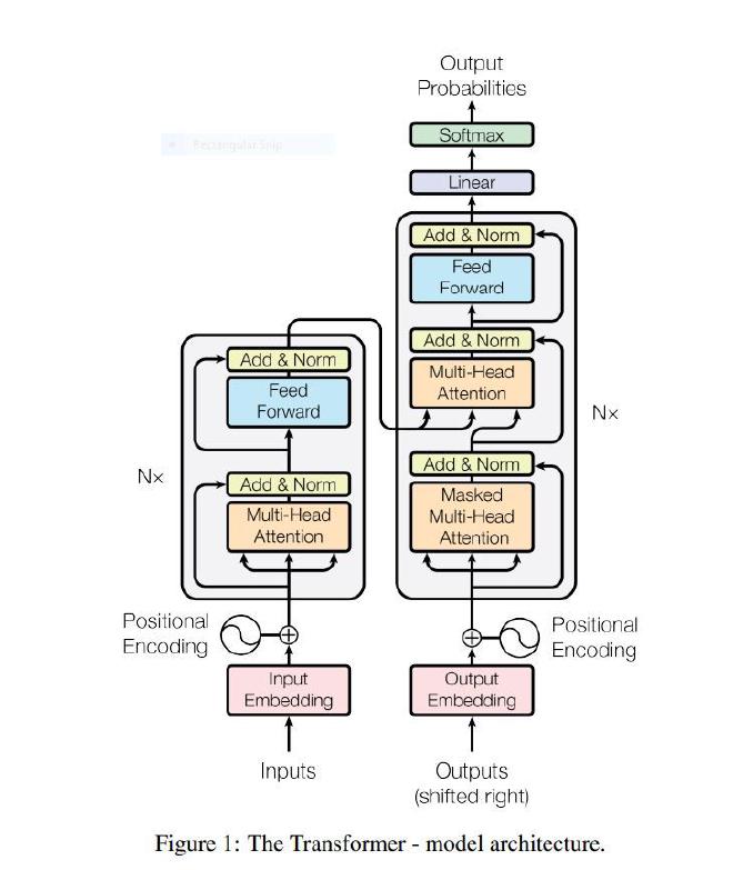
A transformer consists of an encoder and decoder part.
1.1 Encoder #
The encoder’s role is to encode the semantic information of the input in a state (vector). it has \(N_x = 6\) identical layers and each layers has 2 sublayers: multi-head attention and feed forward network.
1.2 Decoder #
The decoder’s role is to generate an output by using the state generated by the encoder.Similarly to the encoder it has \(N_x = 6\) identical layer and each layer has multi-head attention and feed forward network sublayers. But in addition to those 2 sublayers we also have a third one ( the second one on figure 1) which is a multi-head attention layer over the output of the encoder. Moreover the decoder is autogressive meaning it generates one token after another(one word after another) and stops when it reaches the special token EOS(End Of Sequence).
1.3 Input Embedding #
Embedding aims at creating a vector representation of words. Words that have the same meaning will be close in terms of euclidian distance. For the encoder, the authors decided to use an embedding of size dmodel=512 (i.e each word is modeled by a vector of size 512).
2. Attention #
The main purpose of attention is to estimate the compatibility between the keys terms K and the query term Q in a sequence.Think of Q as a search request ,K as a ID matrix of all the word in a sequence and the value V as the actual information content. All of them are vectors of dimension \(d_k\), \(d_k\) and \(d_v\) respectively.
In self attention(also known as intra attention) Q,K and V come from the same input, in other words self attention calculates the importance of a word relative to other words in a specific input.
2.1. Scaled dot product #
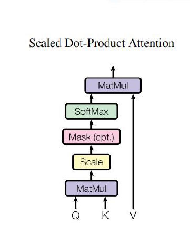
The two most commonly used attention functions are additive attention and dot-product attention. Additive attention computes the compatibility using a feed forward netwrok which is time and ressource consumming. That is the reason why in transformer we use the scaled dot product attention(which comes from dot product attention) that follows this formula
$$ \boxed{\text{Attention}(Q, K, V) = \text{softmax}\left(\frac{Q \times K^T}{\sqrt{d_k}}\right)V} $$we notice that compare to the do product attention we have a special factor \(\frac{1}{\sqrt{d_k}}\).So why this factor? Without this factor, when the dimension \(d_k\) of the vectors becomes large, the value of the dot product \(Q \times K^T\) will also become large. When passed through the softmax function, this can cause saturation, which means the model learns slowly and becomes unstable. The \(\frac{1}{\sqrt{d_k}}\) factor allows the model to control the value of the dot product in order to stabilize the training
2.2. Multi-Head attention #
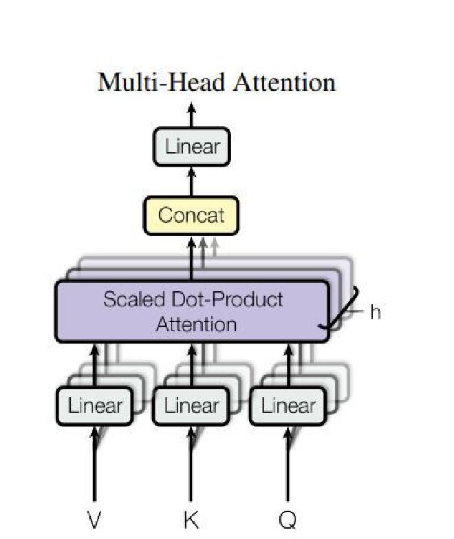
Multi-Head attention allows the transformer to learn different relationships between words.Mathematically it is just a projection of QUERY Q,key K and value V into h linear spaces (h is the number of relation that the transformer learns and it is equal to 8 here)
On each of these projected versions of queries, keys and values we then perform the attention function in parallel(meaning that all the projections are processed at the same time), producing \(d_v\)-dimensional output values. These are concatenated and projected again, which gives the final values, as depicted in Figure 3.
During the training phase, the Multi-Head Attention mechanism has to learn the best projection matrices \(W^Q, W^K, W^V\).
$$ \begin{aligned} \text{MultiHead}(Q, K, V) &= \text{Concat}(\text{head}_1, \dots, \text{head}_h)W^O \\ \end{aligned} $$\(\text{where head}_i = \text{Attention}(QW_i^Q, KW_i^K, VW_i^V)\)
$$ \text{Where the projections are parameter matrices } W_i^Q \in \mathbb{R}^{d_{\text{model}} \times d_k}, W_i^K \in \mathbb{R}^{d_{\text{model}} \times d_k}, W_i^V \in \mathbb{R}^{d_{\text{model}} \times d_v} \text{ and } W^O \in \mathbb{R}^{hd_v \times d_{\text{model}}}. $$The outputs of the Multi-Head Attention mechanism, h attention matrix for each word, are then concatenated to produce one matrix per word. This Attention architecture allows us to learn more complex dependencies between words without adding any training time thanks to the linear projection which reduces the size of each word vector. ( we have 8 projections in space of size 64, 8*64 = 512 the initial size of vector)
As seen previously atention is applied at 3 different levels and for different purposes:
- Encoder level: The query, key and value come from the input embedding .It answers the question how is each word related to others in the input?
- Encoder-Decoder level:The query comes from the decoder part and the key and value come from the encoder part. It answers the question: which words of the input should the decoder focus on to generate the current output?
- Decoder level: The query,key,values come from the decoder. It answers to the question how is each word related to others in the output. Since during the training for a given input we provide the correct output to the encoder in order for it to learn how to correctly predict the ouput ,we have to mask the future in such a way that to predict a current output, the decoder only focuses on previous output,so we use a masked attention meaning that the keys are only related to past output.
3. Position-wise feed forward networks #
In order to extract features and process data we have a fully connected feed-forward network on the decoder and encoder part, which is applied to each position separately and identically. This consists of two linear transformations with a ReLU activation in between.
$$ \boxed{ \text{FFN}(x) = \text{max}(0, xW_1 + b_1)W_2 + b_2\ } $$While the linear transformations are the same across different positions, they use different parameters from layer to layer.The dimensionality of input and output is dmodel = 512, and the inner-layer has dimensionality \(\boxed{d_\text{ff} = 2048}\), W1 has dimension of \(\boxed{d_\text{model} \times d_\text{ff}}\) and W2 has dimension of \(\boxed{d_\text{ff} \times d_\text{model}}\) .
4. positional Encoding(PE) #
Since the transformer contains no recurrence and no convolution, in order for the model to make use of the order of the sequence, the authors of transformer introduce the notion of positional encoding.The positional encoding is a vector that contains information about the position of a specific embedding (word) in a sequence. It is added to the embedding at the bottom of the encoder and decoder stacks. So let us take an example ,without PE a sentence John saw marry doing laundry will be the same as marry saw John doing laundry.
The PE have the same dimension dmodel as the embeddings so that the two can be summed and it uses the following formula :
$$ PE_{(pos, 2i)} = \sin(pos/10000^{2i/d_{\text{model}}})\\ PE_{(pos, 2i+1)} = \cos(pos/10000^{2i/d_{\text{model}}})\ $$where pos is the position and i is the dimension
What is powerful about these formulas is that they allow the model to easily learn relative positions. For example, the shift from position pos to position pos + k can be represented by a linear transformation. Thanks to this, the model can generalize sentences longer than the ones it saw during training. Let us illustrate this through the following example : assume that during the training process of a transformer the maximum length of a sentence was 10 and the model is being tested on a sentence of length 11. To compute the PE of the word at positon 11 the transformer will compute simply compute PE at position 10 and PE at position 1 to induce the word at position 11 as shown below :
$$ \boxed{ \begin{aligned} PE_{(11,2i)} &= \sin((10+1)w)\\ &= \sin(10w)\cos(w) + \sin(w)\cos(10w)\\ &= PE_{(10,2i)}PE_{(1,2i+1)} + PE_{(1,2i)}PE_{(10,2i+1)} \end{aligned} } $$or
$$ \boxed{ \begin{aligned} PE_{(11,2i+1)} &= \cos((10+1)w)\\ &= \cos(10w)\cos(w) - \sin(10w)\sin(w)\\ &= PE_{(10,2i+1)}PE_{(1,2i+1)} - PE_{(10,2i)}PE_{(1,2i)} \end{aligned} } $$\(\text{where}\ w=\frac{1}{10000^{2i/d_{\text{model}}}}\)